Part 3:
Whats going on in the cars brain?
The cars brain How to recognize intentions
- Markov Dynamic Models
- Bayesian networks
- Wellman et al. (1995) Used Bayesian networks (acyclic graphical representation of a joint probability distribution) to determine maneuvers and intentions of vehicles from visual observation of a scene (could be either a camera mounted inside a car, but usually cameras mounted along the highways/bridges and tracking vehicles.
- Fuzzy Logic
- Takahashi (1996) - Fuzzy logic to control drivetrain (automated shifting). Tested on downhill and uphill grades.
- Qiao et al. (1995) - Recognize driving environments (in town, descent) based on pattern matching templates with fuzzy supervisor to account for time variations and changes in vehicle properties.
Expert Systems
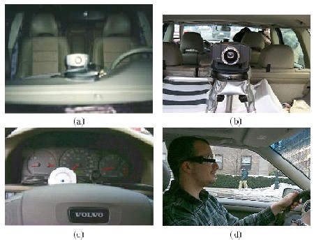
- Malec et al. (1994) - Used a rule-based system to decide the current context of operation to manage information flow in a Volvo for AICC system.
- Niehaus & Stengel (1994) - A combination of rule-based system with a stochastic model of traffic behavior to estimate the behavior of traffic and base future decisions on that information.
Markov Dynamic Model
(Pentland and Liu, 1999)
- Assume each driving action (e.g., passing) is a result of a sequence of internal states.
- Driving actions tend to follow fixed sequence of states -ideal for applying Markov probability structure.
- MDMs describe how a set of dynamic processes must be controlled to generate observed signal.
Assume then that any driving action, such as passing, is actually the result of the driver passing through a sequence of internal states. In this example, assume that there are 3 states (corresponding to prepare, execute, conclude). These large-scale behaviors tend to occur in this fixed sequence, although there can be variations or interruptions. Thus, we can apply a Markov probability structure to connect the states.
Within each state, we can use a dynamic model, such as Kalman filter and control law, to describe the continuous behavior of the driver. So in the passing scenario shown here, the prepare state would have a dynamic model describing how the driver controls the heading and velocity of the car. Thus the MDMs describe how a set of dynamic processes must be controlled in order to generate the observed behavior rather than attempting to describe the behavior directly.
The MDM is conceptually the same as hidden Markov models except that the observations we use are essentially the prediction errors of the dynamic model. In the case of driving then, the observations are roughly the accelerations and heading changes unexplained by the model.
Markov Dynamic Model
This figure now graphically represents a three-state Markov dynamic model for the passing task which is the long-time-scale driving behavior. The circles represent the three states (prepare, execute and conclude) while the arrows represent the Markov transition probabilities between the states. The fourth state is where the driver is simply staying on the road doing nothing, if you will.
Within each of the states of the passing MDM, we can also model the behavior with yet another MDM, here shown by the yellow figures. The models in the individual states dont have to be the same type, as indicated by the two state MDM in the execute state.
To use this method to facilitate the low-level operation of the car during driving, we really want to be able to recognize just the preparatory movements. If this can be done accurately, then the car can anticipate driver behavior for the next several seconds and take appropriate action.
Multiple dynamic model approach
So the next step in recognition is to create a set of MDMs, one model for each of the different possible actions. At each instant, we can then make our observations of the drivers behavior and determine which model best fits the sequence of observations. In our tests, the observations are measurements of the acceleration, and steering angle, and rate of steering angle change. We simply use the expectation-maximization methods traditionally used with HMMs to calculate the likelihoods of the individual models. The model with the maximum likelihood estimate is the one used to classify the current state.
MDM parameter estimation
Parameter estimation for the MDMs is fairly straight forward - just as with HMMs. You need to have a set of examples of the particular driving action and you estimate the transition probabilities and state parameters from the training set using expectation-maximization. The training set can either be the whole action, or as in our case, just the initial preparatory movements (the initial 2 sec of the action).
(In the case of HMMs and what we do, the Viterbi algorithm is used here). There is an interative process that adjusts the parameters to maximize the expected likelihood of generating the set of training examples.
Self-learning configuration
One problem with human drivers is that there are individual differences between drivers. So any modelling approach must be able to tune itself to each individual. One nice feature of this modeling approach is that it is also a self-learning configuration. Over time, the system can adapt itself to each individual.
Assume that weve been able to create a set of generic models of the various driving actions, such as passing, and were actually segmenting driving behavior on-the-fly into the different actions.
Now each example of passing that is segmented, can be incorporated into a new training set.
Now each time you go out for a drive, the car keeps these new training sets in memory. When you get out of the car, it begins the process of re-estimating the parameters of the MDMs to account for the new information. And the next time that you get back in the car, it is a little bit more in tune with your driving behavior.
Recognition of driving actions
Liu and Pentland (1997) use a fixed-base simulator to study recognition of different driving maneuvers.
Kuge et al. (2000) used a motion-base simulator to investigate recognition of normal and emergency braking maneuvers.
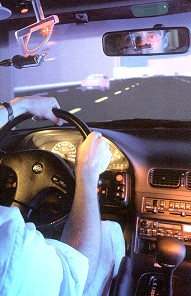
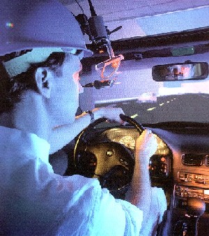
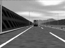
The CBR simulator used by Liu and Pentland (1997) is a fixed base simulator with a single display which is projected onto the wall in front of the simulator. The driver gets a view which is about 60 degrees by 40 degrees vertical. The front part of the car is instrumented to record driver control inputs such as steering angle, brake and accelerator position. The steering wheel also has a motor attached which supplies some torque to imitate steering stiffness and tire slip.
The drivers were instructed to keep a normal speed of 30-35 mph and follow the instructions that appeared on the screen. We recorded the acceleration and steering angle and steering rate at 10 Hz. We later resampled the data at 20Hz, interpolating the intermediate points. We used the appearance of the commands as a way to segment the recording of the whole driving session into the individual actions for the MDM training. We had 8 male subjects, ages 20-40 and each drove for a total of about 20 minutes.
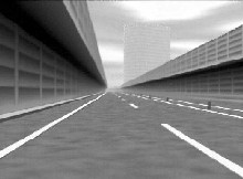
We use the SIRCA simulation which was designed at the Univ. of Valencia in Spain. It is a basic driving simulation, with autonomous vehicles using a rule-based control to keep them driving around. We used a city like environment with only straight roads and intersection.
MDM recognition accuracy
Average recognition accurtacy over all driving tasks (Turning L, Turning R, Stopping, Lane change, Passing, Lane keeping). Maneuver completion ~7.5 sec average.
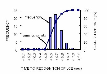
These results from the leave-one-out tests show the recognition accuracy of the MDMs constructed from different lengths of data. All maneuvers are combined in these results. The x-axis is the time after the on-screen command is shown. The y-axis shows the accuracy rate. At 0.5 sec (AFTER RED HATCH AREA), the driver is just beginning to react to the on-screen command. At this point, we only have a 16.7% recognition accuracy (chance level). But after another 1.5 sec, recognition accuracy are up around 95%. The maneuvers averaged ~7.5 secs to complete.
The upper figure illustrates the relative positions of the cars over the time interval of the graph to get a better idea of when recognition takes place. The 2 second point reflect about 20% of the action being completed. Recognition occurs before any big actions occur!
Real-time performance
Recognition rates for various tasks
| | @ 2sec | @ 3sec | @ 4sec |
| Passing: | 67% | 50% | 67% |
| Left turns: | 54% | 50% | 63% |
| Right turns: | 18% | 60% | 70% |
| Stopping: | 4% | 4% | 45% |
| Lane change: | 37% | 18% | 28% |
Accuracy measured as the % correct in 0.5 sec windows starting from the presentation of the on-screen command.
I tried a pilot experiment with three new subjects in the real-time system. (Each one drove the route three times, and we got the following results. These run with models constructed from 2 sec of data.) I looked at the output of the recognizer in a 0.5 second window at the corresponding time after the command. Note the relatively high recognition rates for passing and left turns, and very low rate for stopping. In most cases the accuracy tends to go up with time but lane changes dont quite do that.
In most of the erroneous guesses, the recognizer would often substitute a similar action. For example, if you consider what the drivers had to do for a left turn, most of them would initially slow down. Hence, in many cases, stopping was incorrectly identified as a left turn or right turn. Similarly, lane changes were misclassified as passing in many cases or also as left turns. I suspect that one of the sources of error was in the lower sampling rate, which may cause some sort of aliasing-like problem.
This also suggests that the division of states and protypical actions is not quite right. For example, things like a lane change are more likely to be a particular state or part of a longer-term action like passing. Also shows that context of external environment is really needed.
Recognizing actions - Free driving conditions
- Free driving with free-flowing traffic
- Verbal reporting to segment tasks
- Allows modeling behavior before initiation of maneuver - in essence predicting intentions?
- Preliminary results: Test-on-training set
67.0% @ 2 sec
68.4% @ 3 sec
82.7% @ full duration
One major problem with the previous approach, however, is that most people do not drive their cars based on some command flashing on the screen. So I wanted to test whether we could achieve similar recognition performance under free driving conditions that one would ordinarily expect. Here I used the same road network, but introduced more autonomous cars. Before subjects drove, they were given a list of the actions we wanted them to perform. Then they proceeded to drive in the environment for 10-15 minutes. To segment the data, the drivers were told to verbally report when they started and finished a particular action and the experimenter would record their responses via keyboard into the log file. I didnt explicitly control my definition of the start and finish, but it seemed that most said something just before they started their control movements.
The preliminary results from the test-on training show performance at 67% for models constructed from a 2 second chunk of data (starting from their verbal report). Perfomance increased slightly. For comparison, I tried recognition using MDMs trained on the whole action - here performance is up to a more respectable 82%.
Discriminating lane changes
From Kuge et al. (2000)
Emergency lane changes
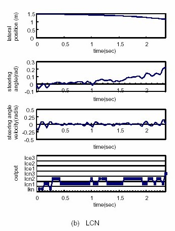
Normal lane changes
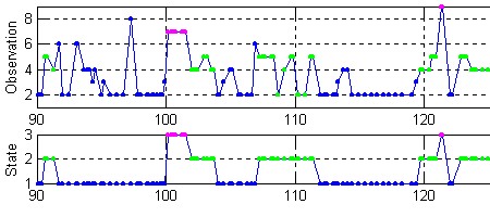
Hidden Markov Model assessment of pilot attention patterns
- Patterns of fixations of the instrument panel indicate the cognitive state or flight task that is currently being performed.
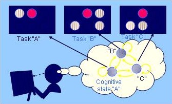
More details can be found in the Eyes Tea presentation by Miwa Hayashi
Recognition using coupled HMMs
From Oliver (2000)
HMMs of driver state and state of surrounding vehicles are coupled to better model the dependencies between them.
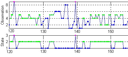
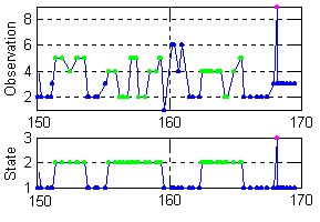
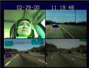
Nuria Oliver did some work on the real roads around Boston using an instrumented vehicle and coupled HMMs to recognize driver actions. She looked at a large set of information including physical state of car in the environment (velocity, acceleration, lane deviation), head pose, facial expressions, road state, traffic state.
She looked at the recognition accuracy of the models (but not in real-time)(performance on the same order as in simulation) and showed an improvement on recognition with environmental information in addition to car state information. Models had good accuracy and could predict the correct task in around 1 sec before any significant deviation (< 20%) in car signals.
Automatic segmentation of the driving scene
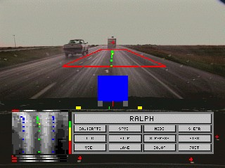
From Pomerleau et al. (1995) Carnegie-Mellon University
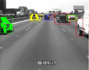
From Malik et al. (1997) University of California, Berkeley
There has been a lot of work at Carnegie Mellon with the NavLab project and at Berkeley with the PATH project to do automatic scene analysis. In fact, this technology is also probably necessary in order to use the eye movements, since there needs to be a segmentation of the scene into different regions.
Drive-away messages
- The drivers eye movements are a potential source of information about the drivers current and intended state/actions.
- There are promising statistical methods for modeling driver behavior that could be implemented in real-time in vehicles.
 But, there are many potential problems to overcome that stem from the complexity of the driving task and, of course, people! But, there are many potential problems to overcome that stem from the complexity of the driving task and, of course, people!
|